


If you want to make your Google Sheets spreadsheet easier to read, you can apply alternate shading to rows or columns. We’ll walk you through it!
Adding Alternate Colors to Rows
You can apply an alternate color scheme to rows in your Google Sheets spreadsheet directly using the “Alternating Colors” formatting feature.
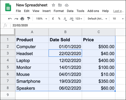
To do so, open your Google Sheets spreadsheet and select your data. You can either do this manually or select a cell in your data set, and then press Ctrl+A to select the data automatically.

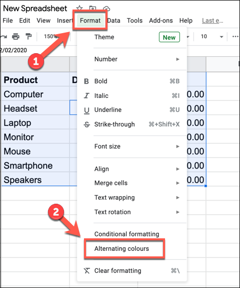
After your data is selected, click Format> Alternating Colors.

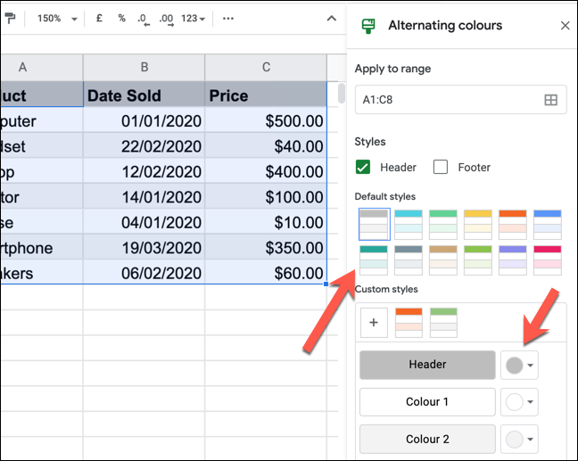
This will apply a basic alternate color scheme to each row of your data set and open the “Alternating Colors” panel on the right, so you can make further changes.
You can also select one of several preset themes, with different alternate colors listed under the “Default Styles” section.
Alternatively, you can create your own custom style by clicking one of the options in the “Custom Styles” section and selecting a new color. You’ll have to repeat this for each color listed.
For instance, if you change the “Header” color, it will also change the color scheme applied to the header row.

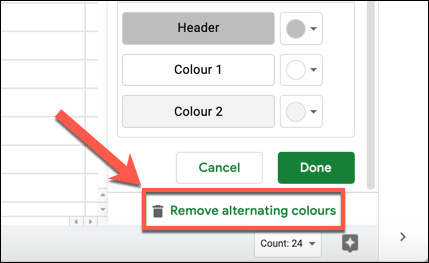
If you want to remove the alternating color scheme from your rows entirely, click “Remove Alternating Colors” at the bottom of the panel.

Adding Alternate Colors to Columns
The “Alternating Colors” feature alternates colors for rows, but won’t do the same for columns. To apply alternate colors to columns, you’ll have to use conditional formatting instead.
To do so, select your data set in your Google Sheets spreadsheet. You can do this manually, or by selecting a cell, and then pressing Ctrl+A to select the data.
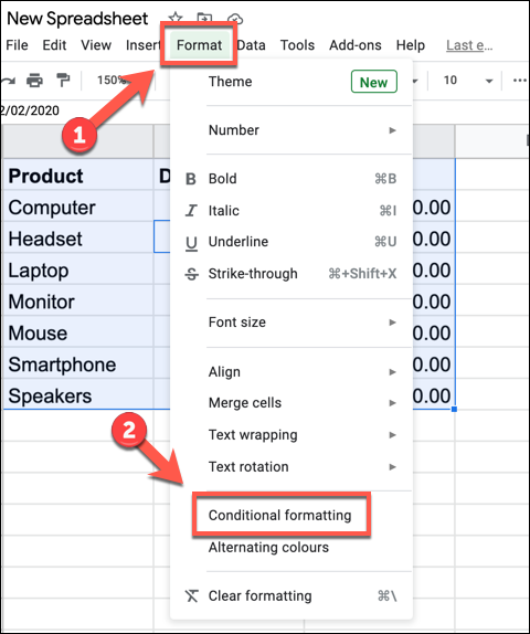
With your data selected, click Format> Conditional Formatting from the menu bar.
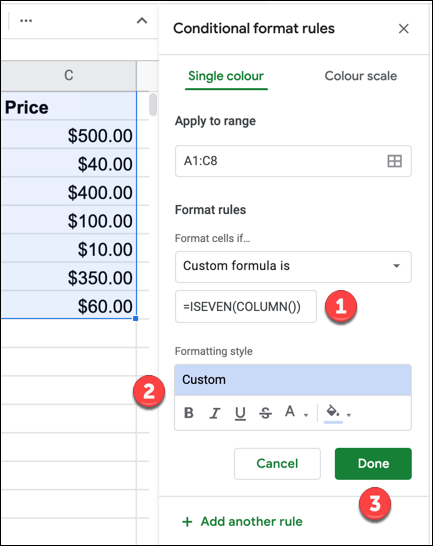
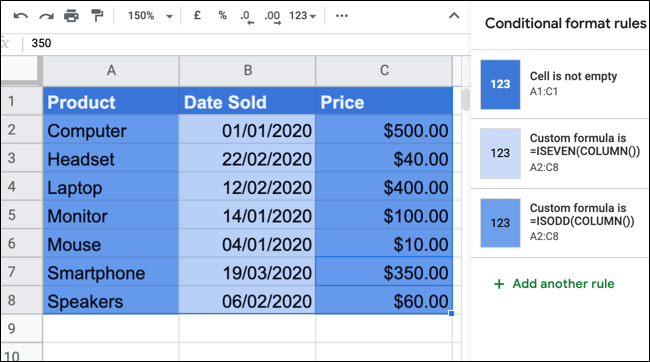
This opens the “Conditional Format Rules” panel on the right. In the “Format Rules” drop-down menu, click “Custom Formula Is.”
In the box below, type the following formula:
=ISEVEN(COLUMN())
Then, select the color, font, and formatting styles you want to apply in the “Formatting Style” box.
Click “Done” to add the rule.

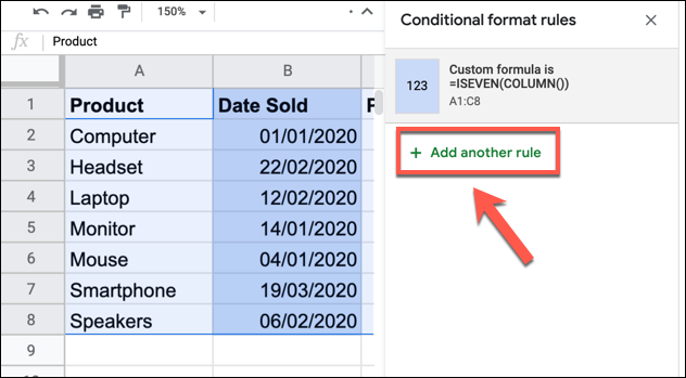
This will apply the formatting options you’ve selected to each column with an even number (column B meaning column 2, column D meaning column 4, and so on).
To add a new formatting rule for odd-numbered columns (column A meaning column 1, column C meaning column 3, and so on), click “Add Another Rule.”

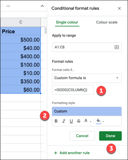
The same as before, select “Custom Formula Is” from the “Format Rules” drop-down menu. In the box provided, type the following:
=ISODD(COLUMN())
Next, select your preferred formatting in the “Formatting Style” options box, and then click “Done.”

After you save, your data set should appear with different formatting for each alternate column.
If you want to apply custom formatting to the header row, you can create a rule to apply formatting on a column row (row 1) first, and then repeat the steps we outlined above for the rest of your data.

This will allow you to tweak the formatting for your header to make it stand out. You can also edit the formatting directly, but conditional formatting rules will override anything you apply.
If you want to edit a conditional formatting rule you’ve applied, click it in the “Conditional Format Rules” panel. You can then remove it entirely by clicking the Delete button that appears whenever you hover over the rule.
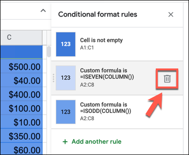

This will immediately remove the conditional formatting rule from your selected data and allow you to apply a new one afterward.

