


The greater the number of rows and columns in your Google Sheets spreadsheet, the more unwieldy it can become. Freezing or hiding rows and columns can make your spreadsheet easier to read and navigate. Here’s how.
Freeze Columns and Rows in Google Sheets
If you freeze columns or rows in Google Sheets, it locks them into place. This is a good option for use with data-heavy spreadsheets, where you can freeze header rows or columns to make it easier to read your data.
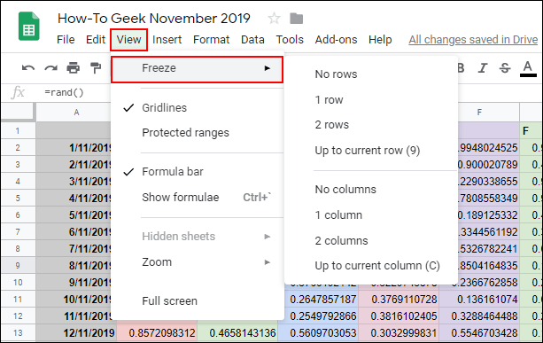
In most cases, you’ll want to freeze only the first row or column, but you can freeze rows or columns immediately after the first. To begin, select a cell in the column or row you’re looking to freeze and then click View> Freeze from the top menu.
Click “1 Column” or “1 Row” to freeze the top column A or row 1. Alternatively, click “2 Columns” or “2 Rows” to freeze the first two columns or rows.
You can also click “Up to Current Column” or “Up to Current Row” to freeze the columns or rows up to your selected cell.

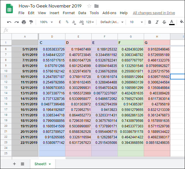
When you move around your spreadsheet, your frozen cells will remain in place for you to easily refer back to.
A thicker, gray cell border will appear next to a frozen column or row to make the border between your frozen and unfrozen cells clear.

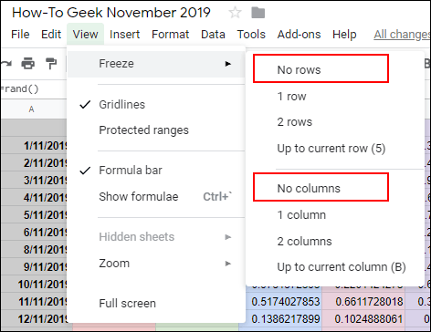
If you want to remove frozen columns or rows, click View> Frozen and select “No Rows” or “No Columns” to return these cells to normal.

Hide Columns and Rows in Google Sheets
If you want to temporarily hide certain rows or columns, but don’t want to remove them from your Google Sheets spreadsheet completely, you can hide them instead.
Hide Google Sheets Columns
To hide a column, right-click the column header for your chosen column. In the menu that appears, click the “Hide Column” button.
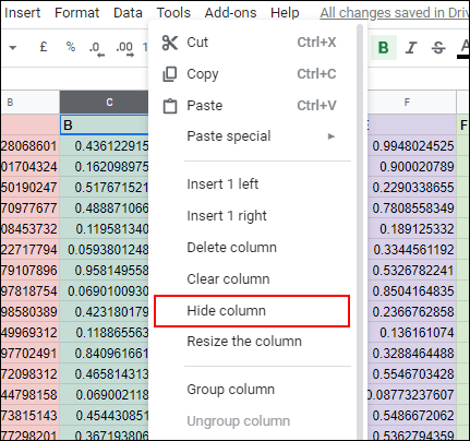

Your column will then disappear from view, with arrows appearing in the column headers on either side of your hidden column.


Clicking on these arrows will expose the column and return it to normal. Alternatively, you can use keyboard shortcuts in Google Sheets to hide your column instead.
Click the column header to select it and then press Ctrl+Alt+0 on your keyboard to hide it instead. Selecting the columns on either side of your hidden row and then pressing Ctrl+Shift+0 on your keyboard will unhide your column afterward.
Hide Google Sheets Rows
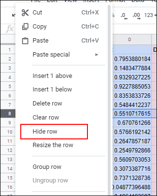
Similar to the process above, if you want to hide a row in Google Sheets, right-click on the row header for the row you’re looking to hide.
In the menu that appears, click the “Hide Row” button.

Your selected row will disappear, with opposite arrows appearing in the header rows on either side.
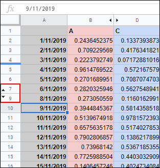

Click on these arrows to display your hidden row and return it to normal at any point.
If you’d prefer to use a keyboard shortcut, click the row header to select it and then press Ctrl+Alt+9 to hide the row instead. Select the rows on either side of your hidden row and press Ctrl+Shift+9 on your keyboard to unhide it afterward.

