


No matter how careful you are entering or importing data, duplicates can happen. While you could find and remove duplicates, you may want to review them, not necessarily remove them. We’ll show you how to highlight duplicates in Google Sheets.
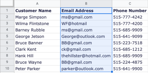
You may have a list of customer email addresses and phone numbers, product identifiers and order numbers, or similar data where duplicates shouldn’t exist. By locating and highlighting duplicates in your spreadsheet, you can then review and fix the incorrect data.


While Microsoft Excel offers an easy way to find duplicates with conditional formatting, Google Sheets doesn’t currently provide such a convenient option. But with a custom formula in addition to the conditional formatting, highlighting duplicates in your sheet can be done in a few clicks.
Find Duplicates in Google Sheets by Highlighting Them
Sign in to Google Sheets and open the spreadsheet you want to work with. Select the cells where you want to find duplicates. This can be a column, row, or cell range.

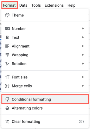
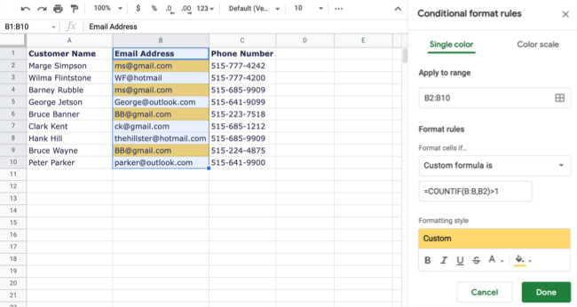
Click Format> Conditional Formatting from the menu. This opens the Conditional Formatting sidebar where you’ll set up a rule to highlight the duplicate data.

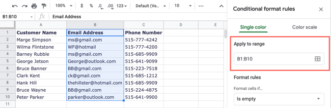
At the top of the sidebar, select the Single Color tab and confirm the cells beneath Apply to Range.

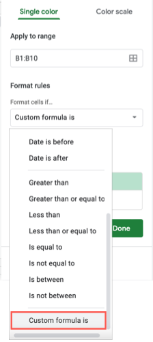
Below Format Rules, open the drop-down box for Format Cells If and select “Custom Formula Is” at the bottom of the list.

Enter the following formula into the Value or Formula box that displays beneath the drop-down box. Replace the letters and cell reference in the formula with those for your selected cell range.
=COUNTIF(B:B,B1)>1
Here, COUNTIF is the function, B:B is the range (column,) B1 is the criteria, and >1 is more than one.
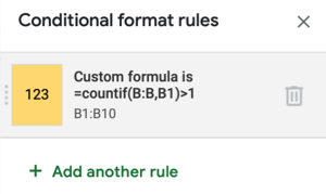
Alternatively, you can use the following formula for exact cell references as the range.
=COUNTIF($B$1:$B$10,B1)>1
Here, COUNTIF is the function, $B$1:$B$10 is the range, B1 is the criteria, and >1 is more than one.
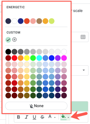
Under Formatting Style, choose the type of highlight you want to use. You can use the Fill Color icon to choose a color from the palette. Alternatively, you can format the font in the cells with bold, italic, or a color if you prefer.

Click “Done” when you finish to apply the conditional formatting rule. You should see the cells containing duplicate data formatted with the style you selected.

As you make corrections to the duplicate data, you’ll see the conditional formatting disappear leaving you with the remaining duplicates.
Edit, Add, or Delete a Conditional Formatting Rule
You can make changes to a rule, add a new one, or delete a rule easily in Google Sheets. Open the sidebar with Format> Conditional Formatting. You’ll see the rules you’ve set up.
- To edit a rule, select it, make your changes, and click “Done.”
- To set up an additional rule, select “Add Another Rule.”
- To remove a rule, hover your cursor over it and click the trash can icon.

By finding and highlighting duplicates in Google Sheets, you can work on correcting the wrong data. And if you’re interested in other ways to use conditional formatting in Google Sheets, look at how to apply a color scale based on value or how to highlight blanks or cells with errors.

